Calculate Camera Exposure Times for Scientific Photography

Calculate camera exposure times using the formula ET = (LN / (ISO * AP²)) * 100, where LN is luminance, ISO is sensitivity, and AP is aperture. You’ll need to balance these variables while aiming to maximize dynamic range without causing pixel saturation. For scientific photography, start with ISO 400 as your baseline, then adjust exposure times based on your brightest sample. Monitor histograms to keep intensity levels below maximum values. The techniques below will help you capture scientifically accurate images with ideal clarity.

13 Second-Level Headings for “Calculate Camera Exposure Times for Scientific Photography”

How do you make certain your scientific images are perfectly exposed every time? By understanding the key components that affect exposure calculation. Your article should include these essential headings:

Scientific imaging demands perfect exposure—mastering the exposure formula is your key to consistent, publishable results.

1. Understanding the Exposure Formula
2. Measuring Luminance Accurately
3. Selecting Appropriate ISO Values
4. Optimizing Aperture Settings
5. Calculating Long Exposure Times
6. Ensuring Consistency Across Samples

Each section should explain how these factors influence the ET = (LN / (ISO * AP^2)) * 100 formula.

When you’re working with low-light specimens, you’ll need to calculate long exposure times precisely to avoid under or overexposure.

Remember that wider apertures (lower f-stops) can greatly reduce the exposure time needed, while higher ISO values offer speed at the cost of image noise.

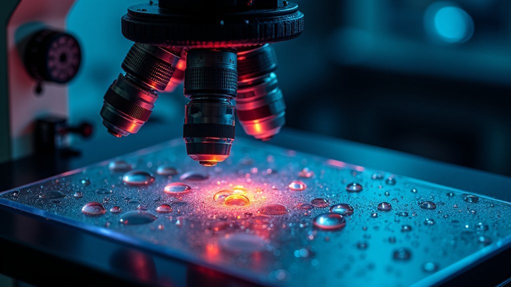
Fundamentals of Microscope Camera Exposure

Three vital elements define successful microscope photography: proper exposure time, stable specimen preparation, and appropriate camera settings.

When you’re capturing microscopic specimens, the exposure time directly impacts image quality by determining how much light reaches your sensor.

Finding the ideal exposure requires balancing sufficient light capture against potential motion blur. Calculate your perfect time using the formula ET = (LN / (ISO * AP^2)) * 100, which accounts for luminance, ISO sensitivity, and aperture.

For live cell imaging, shorter shutter speed is essential to minimize photodamage while still capturing important details.

Maintain consistent exposure times when comparing control and experimental samples to guarantee scientific validity.

Using software to monitor pixel intensity during image capture helps you achieve both aesthetic quality and scientific accuracy without compromising your data.

Essential Variables Affecting Exposure Calculations

When calculating ideal camera exposure time for scientific imaging, you’ll need to account for light intensity variables including scene luminance and aperture settings, which directly control the amount of light reaching your sensor.

Your camera’s ISO setting determines sensor sensitivity, creating a three-way relationship where higher sensitivity allows for shorter exposure times but potentially introduces image noise.

Light Intensity Variables

While capturing precise scientific images requires technical skill, understanding the essential variables affecting exposure calculations forms the foundation of successful scientific photography.

Light intensity, measured in luminance (cd/m²), directly impacts how your camera sensor captures images and determines appropriate exposure time.

When calculating ideal exposure settings, consider these key light intensity factors:

1. Luminance levels – Higher luminance reduces required exposure time, while lower light conditions necessitate longer exposures.
2. Camera sensor sensitivity – Your ISO setting determines how quickly your sensor responds to available light.
3. Aperture settings – Lower f-stops allow more light to reach your sensor, enabling shorter exposure times.

Using the formula ET = (LN / (ISO AP²)) 100, you’ll achieve precise control over your scientific imaging results by balancing these critical variables.

Sensor Sensitivity Considerations

Your camera’s sensitivity setting creates a mathematical trade-off: doubling the ISO halves the necessary exposure time for identical lighting conditions.

This relationship becomes essential when photographing light-sensitive specimens or rapidly changing phenomena. However, remember that elevated sensitivity often introduces noise into your images, potentially obscuring fine details.

For precise scientific documentation, you’ll need to balance ideal exposure times against image quality requirements.

Input your camera’s ISO value accurately when using exposure calculators to guarantee your results maintain both proper exposure and scientific integrity.

The Mathematics Behind Exposure Time Formulation

The mathematics of exposure time follows the formula ET = (LN / (ISO * AP²)) * 100, giving you a precise starting point for scientific photography.

You’ll need to optimize your dynamic range by setting exposure times that prevent pixel saturation while capturing the full intensity spectrum of your samples.

When working with varying sample brightness, you can adjust this calculation through strategic trial exposures, ensuring you’re capturing meaningful data rather than over or underexposed images.

Exposure Time Calculation Formula

Three critical factors affect your exposure calculation:

1. Luminance (cd/m²) – measures the light intensity reflected from your subject.
2. ISO sensitivity – higher values reduce required exposure time but may introduce noise.
3. Aperture (f-stop) – squared in the formula because its area, not diameter, determines light entry.

Mastering this formula guarantees your scientific photographs achieve ideal brightness without sacrificing detail or accuracy.

Dynamic Range Optimization

You’ll need to calibrate your exposure time based on the brightest expected signal in your sample group. This prevents pixel saturation that can obscure critical details in high-intensity regions.

When your ET is correctly calculated, your camera captures the full spectrum of light intensities present in your specimen.

Don’t hesitate to adjust settings through trial and error, especially with unevenly stained samples.

Monitor your histogram or intensity indicators during imaging to verify you’re capturing the complete dynamic range.

This mathematical approach guarantees your scientific photographs maintain detail integrity across all luminance levels.

Optimizing Dynamic Range in Microscopy Imaging

When capturing microscopy images with scientific precision, properly optimizing the dynamic range becomes essential for meaningful results. You’ll need to calibrate your exposure time based on the brightest expected signal in your sample to prevent pixel saturation and utilize your camera’s full capabilities.

For ideal results:

1. Set exposure time using your brightest sample first, ensuring no pixels reach saturation while maximizing signal-to-noise ratio.
2. Use shorter exposure times for live-cell imaging to maintain cell viability while still capturing necessary details and structure.
3. Monitor pixel intensity through histogram displays in your imaging software to confirm you’re capturing the full dynamic range without clipping.

Maintaining consistent exposure settings between control and treated samples is critical when making intensity comparisons—always select the longest non-saturating exposure time for all comparable images.

Specimen-Specific Exposure Considerations

Different specimens require tailored exposure strategies to capture their unique characteristics accurately.

Begin by identifying your brightest sample to establish baseline exposure times that prevent pixel saturation while maximizing dynamic range. This approach guarantees accurate representation across all specimens.

For unevenly stained samples, you’ll need to experiment with exposure settings until you achieve the desired visual outcome.

When working with live cells, prioritize shorter exposures to minimize phototoxicity while still capturing essential details.

When comparing treated and control samples, maintain consistent exposure times across all specimens for reliable intensity comparisons. This practice highlights true differences in treatment effects rather than artificial variations from changing exposure settings.

For aesthetic purposes, set your exposure to utilize your camera’s full dynamic range without overexposing any critical features.

Preventing Pixel Saturation in Bright Field Microscopy

Setting your exposure time based on the brightest areas of your specimen provides an ideal baseline for capturing detailed bright field images without saturation.

You’ll want to monitor your pixel intensity levels in real-time using your imaging software’s histogram function to immediately identify when saturation occurs.

Optimal Exposure Baselines

Establishing appropriate exposure times forms the cornerstone of successful bright field microscopy imaging.

You’ll need to identify the sample with the brightest signal and adjust your settings accordingly to prevent pixel saturation that can distort image quality.

To determine suitable exposure baselines:

1. Set exposure time long enough to capture sufficient detail while keeping maximum pixel intensity below saturation levels.
2. Utilize visual indicators like histograms to verify you’re effectively using your camera’s full dynamic range.
3. Maintain consistent exposure settings across all images when comparing treated and control samples.

Regular calibration with reference samples will help you determine ideal settings for your specific microscopy conditions.

This disciplined approach guarantees variations in intensity reflect true biological differences rather than artifacts from inconsistent imaging parameters.

Real-time Saturation Monitoring

While baseline exposure settings provide a foundation for quality imaging, active monitoring during acquisition serves as your safeguard against data loss.

Modern imaging software displays real-time pixel intensity levels and histograms that help you prevent exceeding the saturation threshold during exposure.

Watch for visual indicators on your camera that alert you when pixel values approach the maximum (255 for 8-bit images).

You’ll need to adjust exposure times based on the brightest expected signal in your sample, setting them just long enough to capture necessary details while keeping bright regions below saturation levels.

For consistent results, regularly calibrate your imaging system and maintain consistent exposure settings.

This approach guarantees you’re capturing the full dynamic range of your specimen without losing valuable data to overexposure.

Fluorescence Imaging Exposure Requirements

Because fluorescence signals vary dramatically in intensity across different samples, proper exposure time settings can make or break your scientific imaging.

You’ll need to find a delicate balance between capturing sufficient signal and avoiding pixel saturation, especially when dealing with dimly fluorescent specimens.

When setting up your fluorescence imaging protocol:

1. Start with trial exposures targeting the brightest area of your sample while monitoring histogram data to prevent saturation.
2. Maintain identical exposure times between control and experimental groups to guarantee valid quantitative comparisons.
3. Minimize exposure times for live-cell experiments to reduce phototoxicity while still utilizing your camera’s full dynamic range.

Remember that consistent exposure settings are fundamental for accurate data interpretation, particularly when comparing fluorescence intensities between different experimental conditions.

Live Cell Imaging Exposure Limitations

Since living cells are highly sensitive to light damage, your exposure times must be carefully restricted when conducting live cell imaging. Aim for exposure durations in fractions of a second to preserve cell viability while still capturing necessary details.

Live cells require minimal light exposure—use sub-second durations to maintain viability while acquiring essential data.

You’ll need to calibrate exposure based on the brightest signals in your sample, preventing pixel saturation while maintaining sufficient detail. Don’t sacrifice cell health for brighter images—focus instead on capturing essential cellular structures.

Monitor pixel intensity through your imaging software to avoid overexposure, which can be particularly harmful to live specimens. This often requires some trial and error as you balance ideal exposure time against the specific characteristics of your sample and imaging objectives.

Remember that maintaining cell integrity should always take priority over aesthetic image qualities.

Comparative Analysis Exposure Techniques

When conducting comparative analyses between samples, your exposure settings become critical instruments for scientific validity rather than merely technical choices.

You’ll need to select the longest possible exposure time that avoids pixel saturation across all samples to guarantee accurate intensity comparisons.

For scientifically sound comparisons, follow these guidelines:

1. Maintain consistency – Use identical exposure settings for all samples in your comparative study, even if some appear dimmer.
2. Maximize signal – Push exposure times to the threshold before saturation occurs in your brightest sample.
3. Document settings – Record all parameters including exposure time, gain, and binning for reproducibility.

Unlike aesthetic imaging where you optimize for visual appeal, comparative analysis requires standardized conditions to generate quantifiable data that accurately reflects biological differences rather than technical variations.

Practical Exposure Time Calculator Tools

Several powerful calculator tools now exist to eliminate guesswork from your exposure time decisions in scientific photography. Applications like SharpCap and N.I.N.A. allow you to input specific camera parameters and current sky conditions to determine ideal exposure settings with precision.

Steve Bellavia’s specialized CMOS camera spreadsheets incorporate Noise Tolerance Factor (C) for enhanced accuracy in exposure calculations. You’ll find community-shared calculators tailored for various Bortle sky levels particularly valuable when adapting to different imaging locations.

Many modern calculators analyze data in real-time, automatically adjusting to changing environmental conditions throughout your imaging session.

Compensating for Light Source Variations

Scientific photographers regularly confront the challenge of varying light intensities across different imaging scenarios.

To maintain consistent image quality while working with different light sources, you’ll need to adjust your exposure times proportionally to luminance values.

1. Adjust exposure inversely to brightness – Brighter sources require shorter exposures to prevent saturation, while dimmer sources need longer exposures to capture sufficient detail.
2. Monitor your histogram – Use your camera’s histogram display for real-time feedback on pixel intensity and saturation levels, allowing you to quickly adjust exposure times as lighting conditions change.
3. Maintain consistent aperture settings – Keep your aperture value (AP) uniform across different exposures to guarantee comparable depth of field and light entry, making your scientific images more reliable for analysis and comparison.

Relationship Between ISO, Aperture, and Exposure in Microscopy

Mastering microscopy photography requires a thorough understanding of the exposure triangle – the interdependent relationship between ISO, aperture, and exposure time. When you adjust one parameter, you’ll need to compensate with others to maintain proper exposure.

Higher ISO settings increase your sensor’s light sensitivity, allowing shorter exposure times without sacrificing brightness. However, this can introduce noise. Meanwhile, a wider aperture (lower f-stop) permits more light to reach your sensor, also enabling reduced exposure times.

Understanding the tradeoffs: higher ISO means more light sensitivity but potential noise, while wider apertures allow more light but affect depth of field.

For scientific microscopy, start with ISO 400 and f/8 aperture as baseline settings. From there, calculate your exposure time based on sample brightness to avoid pixel saturation while maximizing dynamic range.

The goal is to balance these settings to capture clear, detailed images with minimal noise and ideal light capture.

Frequently Asked Questions

How to Calculate Exposure Time in Photography?

Calculate exposure time using ET = (LN / (ISO * AP^2)) * 100. You’ll need to know the luminance, ISO, and aperture. Monitor for pixel saturation and adjust through trial and error for best results.

How Do You Find the Exposure Time of a Photo?

You’ll find exposure time by measuring luminance, setting ISO and aperture, then using ET = (LN/(ISO*AP²))*100. Check pixel intensity through software histograms and adjust through trial and error for ideal brightness without saturation.

How to Calculate Pinhole Exposure Time?

To calculate pinhole exposure time, divide your focal length by hole diameter to find the pinhole number, take a light meter reading at f/22, then square the ratio of pinhole number to f/22 for your exposure time.

What Is the Camera Exposure Equation?

The camera exposure equation is ET = (LN / (ISO * AP^2)) * 100, where ET is exposure time in seconds, LN is luminance, ISO is sensitivity, and AP is aperture value in f-stop.

In Summary

You’ve now mastered the fundamentals of calculating precise exposure times for scientific photography. By understanding the interplay between ISO, aperture, and light source variations, you’ll capture specimens with ideal dynamic range and detail. Remember that exposure calculation isn’t just mathematics—it’s an essential skill that elevates your microscopy imaging from merely adequate to truly exceptional. Apply these techniques consistently, and you’ll produce publication-quality scientific images every time.